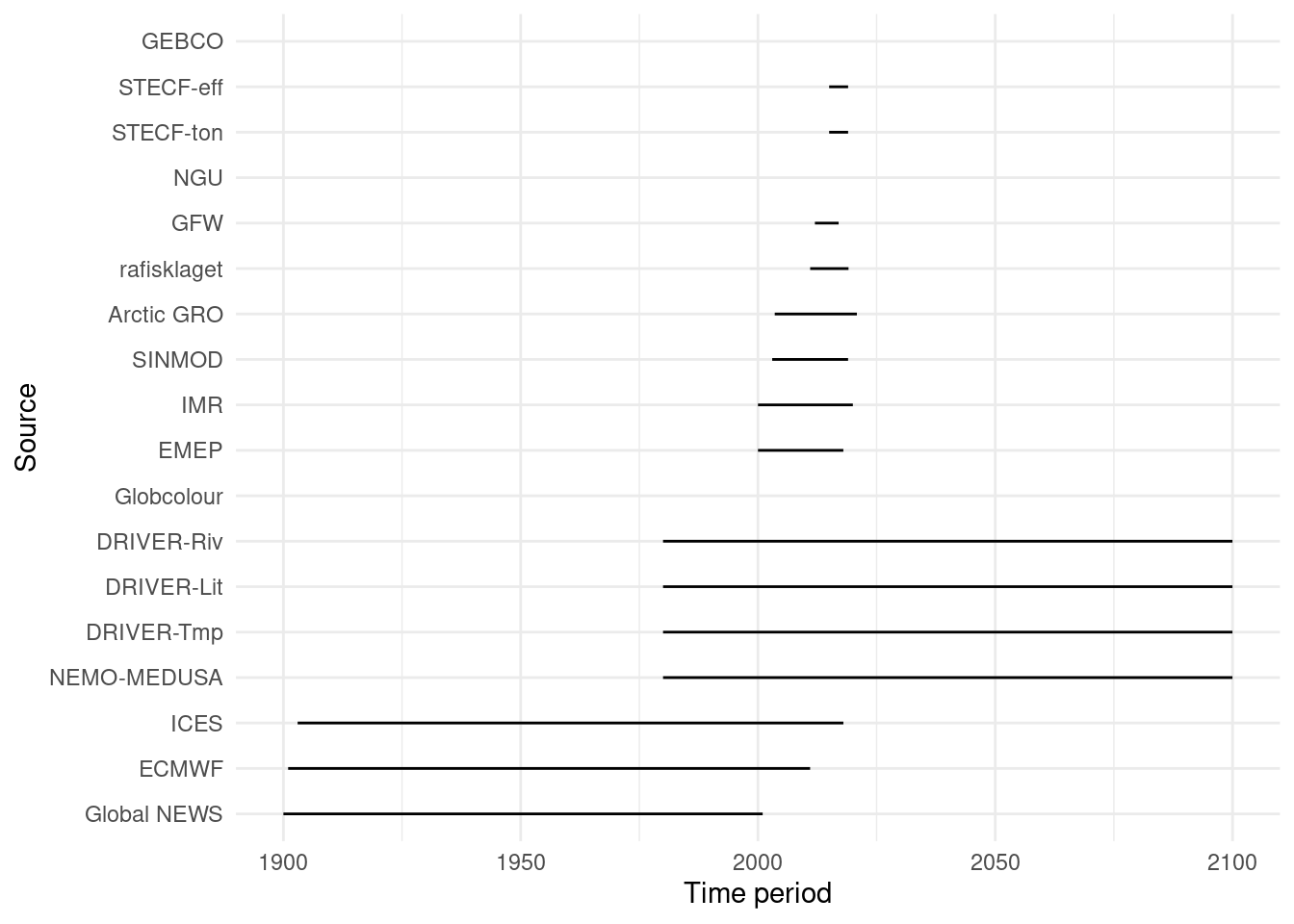
Data Sources
Below is a record of the data products synthesised during MiMeMo. I’ve kept track of the structure of the data to make it easier to quickly check what we have. This will also function as a README for anyone else who follows and wants signposting to sources, or to know what additional data could be downloaded.
NEMO-MEDUSA
Light
Shortwave surface Irradiance inputs to NEMO-MEDUSA.
Source
Available on the idrive at Strathclyde, supplied by Andy Yool at NOC.
Space
Global.
Time
- From 01/01/1980.
- To 28/12/2099.
- In 6 hours.
File structure
- 120 netcdf files.
- 4.5gb total memory requirment.
- 1 netcdf file contains a 2D spatial grid and all timesteps within a year.
Target vars
- ‘SWF’, Total downward short wave flux, or surface irradiance (W per m2 per day). A Watt per m2 is equivalent to a joule per m2 per second.
Spatial vars
- ‘latitude’, vector of latitudes as a file dimension (rectilinear grid).
- ‘longitude’, vector of longitudes as a file dimension (rectilinear grid).
other vars
NA
Air Temperature
Surface air temperatures as inputs to NEMO-MEDUSA.
Source
Available on the idrive at Strathclyde, supplied by Andy Yool at NOC.
Space
Global.
Time
- From 01/01/1980.
- To 28/12/2099.
- In day.
File structure
- 120 netcdf files.
- 17.9gb total memory requirement
- 1 netcdf file contains a 2D spatial grid and all timesteps within a year.
Target vars
- ‘T150’, Air temperature at 1.5 m elevation (K).
Spatial vars
- ‘latitude’, vector of latitudes as a file dimension (rectilinear grid).
- ‘longitude’, vector of longitudes as a file dimension (rectilinear grid).
other vars
NA
Rivers
Freshwater inputs to NEMO-MEDUSA.
Source
Available on the idrive at Strathclyde, supplied by Andy Yool at NOC.
Space
Global.
Time
- From 01/01/1980.
- To 28/12/2099.
- In month.
File structure
- 120 netcdf files.
- 1.3gb total memory requirement.
- 1 netcdf file contains a 2D spatial grid and all timesteps within a year.
Target vars
- ‘sorunoff’, Water runoff from land to sea (Kg per m2 per second).
Spatial vars
- ‘nav_Lat’, Matrix of latitudes (curvilinear grid).
- ‘nav_Lon’, Matrix of longitudes (curvilinear grid).
other vars
NA
Model output
NEMO-MEDUSA model OUTPUTS for multiple Variables.
Source
Available on the idrive at Strathclyde, supplied by Andy Yool at NOC.
Space
North Atlantic into Arctic..
Time
- From 01/01/1980.
- To 28/12/2099.
- In 5 days.
File structure
- 51840 netcdf files.
- 543gb total memory requirement.
- Files are organised into folders by year. There are 5 types of file per year, each contains a different set of variables for one time step.
Target vars
- grid_T files:
- ‘soicecov’, Ice fraction (0-1).
- ‘vosaline’, Salinity (psu).
- ‘votemper’, Water temperature (C).
- grid_U files:
- ‘vozocrtx’, Zonal current speed (m per second).
- grid_V files:
- ‘vomecrty’, Meridional current speed (m per second).
- grid_W files:
- ‘votkeavt’, Vertical eddy diffusivity (m2 per second).
- icemod files:
- ‘ice_pres’, Ice presence (logical).
- ‘isnowthi’, Snow thickness (m).
- ‘iicethic’, Ice thickness (m).
- ptrc_T files:
- ‘PHN’, Non-diatom phytoplankton (mmol N per m3).
- ‘PHD’, Diatom phytoplankton (mmol N per m3).
- ‘DIN’, Dissolved inorganic nitrogen (mmol N per m3).
- ‘DET’, Detritus (mmol N per m3).
Spatial vars
❗ Note, these matrices are different for velocity files (cell corners not centres). The grid otherwise appears the same.
❗ Note, grid_W files contain different depths for layers.
- ‘nav_Lat’, Matrix of latitudes for freshwater input (curvilinear grid).
- ‘nav_Lon’, Matrix of longitudes for freshwater input (curvilinear grid).
- ‘deptht’, Vector of depths as a dimension.
other vars
- grid_T files:
- ‘sossheig’, Sea surface height (m).
- grid_W files:
- ‘vovecrtz’, Ocean vertical velocity (m per second).
- icemod files:
- ‘iicevelu’, Ice zonal velocity (m per second).
- ‘iicevelv’, Ice meridional velocity (m per second).
- ptrc_T files:
- ‘CHN’, Chl-a concentration in non-diatom phytoplankton (mg per m3).
- ‘CHD’, Chl-a concentration in diatom phytoplankton (mg per m3).
- ‘ZMI’, Micro-zooplankton (mmol N per m3).
- ‘ZME’, Meso-zooplankton (mmol N per m3).
- ‘SIL’, Silicate (mmol Si per m3).
Other Ecological Drivers
GEBCO
Global terrain model for ocean and land at 15 arc-second intervals.
Space
Global.
Time
- From 01/01/2019.
- To NA.
- In NA.
File structure
- 1 netcdf
- 11gb total memory requirement.
- The file contains a global 2D spatial grid.
Target vars
- ‘elevation’, Bathymetry and topography.
Spatial vars
- ‘lat’, vector of latitudes (rectilinear grid).
- ‘lon’, vector of longitudes (rectilinear grid).
other vars
NA
NGU
Sediment classes in the Barents Sea, an overview document of likely bottom types from expert synthesis of multiple data sets (‘SEABED SEDIMENTS (GRAIN SIZE), N750 OVERVIEW’).
Space
Barents Sea. .
Time
- From 01/01/2015.
- To NA.
- In NA.
File structure
- 1 shape file.
- 8mb total memory requirement.
- The file contains a collection of spatial polygons where sediment classes are expected to occur within the Barents Sea.
Target vars
- ‘SEDKORNSTR’, Sediment grain size code.
- ‘SEDKO_NAVN’ , Sediment grain size class name.
Spatial vars
Polygon boundaries embedded in shapefile.
other vars
NA
ECMWF
Significant wave height and direction from the CERA-20C ‘Ocean Wave Synoptic Monthly Means’.
Space
I downloaded the Northern hemisphere only.
Global.
Time
- From 01/01/1901.
- To 28/12/2010.
- In 3 hours.
File structure
I only downloaded as far back as 2000.
- 11 netcdf files.
- 78.3gb total memory requirement.
- 1 netcdf file contains a 2D spatial grid and all timesteps within a year.
Target vars
- ‘swh’, Mean significant wave height (m).
- ‘mwd’, Mean wave direction (degrees).
- ‘mwp’, Mean wave period.
Spatial vars
Located within netcdf dims, not as variables.
- ‘latitude’, vector of latitudes (rectilinear grid).
- ‘longitude’, vector of longitudes (rectilinear grid).
other vars
Additional variables are available, but have not been downloaded from the web portal.
‘10 metre wind direction’, ‘10 metre wind speed’, ‘Air density over the oceans’, ‘Benjamin-Feir index’, ‘Coefficient of drag with waves’, ‘Free convective velocity over the oceans’, ‘Maximum individual wave height’, ‘Mean direction of total swell’, ‘Mean direction of wind waves’, ‘Mean period of total swell’, ‘Mean period of wind waves’, ‘Mean square slope of waves’, ‘Mean wave direction of first swell partition’, ‘Mean wave direction of second swell partition’, ‘Mean wave direction of third swell partition’, ‘Mean wave period based on first moment’, ‘Mean wave period based on first moment for swell’, ‘Mean wave period based on first moment for wind waves’, ‘Mean wave period based on second moment for swell’, ‘Mean wave period based on second moment for wind waves’, ‘Mean wave period of first swell partition’, ‘Mean wave period of second swell partition’, ‘Mean wave period of third swell partition’, ‘Mean zero-crossing wave period’, ‘Normalized energy flux into ocean’, ‘Normalized energy flux into waves’, ‘Normalized stress into ocean’, ‘Peak wave period’, ‘Period corresponding to maximum individual wave height’, ‘Significant height of total swell’, ‘Significant height of wind waves’, ‘Significant wave height of first swell partition’, ‘Significant wave height of second swell partition’, ‘Significant wave height of third swell partition’, ‘U-component stokes drift’, ‘V-component stokes drift’, ‘Wave Spectral Skewness’, ‘Wave spectral directional width’, ‘Wave spectral directional width for swell’, ‘Wave spectral directional width for wind waves’, ‘Wave spectral kurtosis’, ‘Wave spectral peakedness’.
SINMOD
Tidally resolved water velocity fields in the Arctic. Numerical ocean model output.
Source
Available on the idrive at Strathclyde, supplied by Ingrid Ellingsen at SINTEF
Space
Arctic.
Time
- From 01/01/2003.
- To 28/12/2018.
- In 336 timesteps (every 2 hours in a 28 day month)..
File structure
- 191 netcdf files.
- 600gb total memory requirement.
- 1 netcdf file contains a 3D spatial grid and all timesteps within a month.
Target vars
- ‘u_east’, Zonal veolcity.
- ‘v_north’, Meridional velocity.
Spatial vars
- ‘gridLats’, matrix of latitudes (curvilinear grid).
- ‘gridLons’, matrix of longitudes (curvilinear grid).
- ‘depths’, matrix of depths.
- ‘ldepths’, vector of depth layer thicknesses?
other vars
w_east’, ‘w_north’, ‘w_velocity’, ‘vertical_diffusivity’, ‘NO3’, ‘PhytoF’, ‘PhytoD’, ‘temperature’, ‘salinity’, ‘ice_thickness’, ‘ice_compactness’, ‘freezing_rate’, ‘salinity_ice’, ‘uIce_east’, ‘vIce_north’, ‘uUnderIceE’, ‘vUnderIceN’, ‘elevation’.
Global NEWS
‘Global Nutrient Export from Watersheds’. Modeled N and P input to oceans from rivers.
Space
Global.
Time
- From 01/01/1900.
- To 28/12/2000.
- In 5 years.
- Duration Updated annually.
File structure
- 3 csv files.
- 6mb total memory requirement.
- The files contain river mouth coordinates, Nitrogen loads, river discharge volume.
Target vars
- ‘Nload’, Nitrogen reaching the sea from a river (kg per year).
- ‘Discharge’, Water volume released at the river mouth (km3 per year).
Spatial vars
- ‘lat’, vector of latitudes (rectilinear grid).
- ‘lon’, vector of longitudes (rectilinear grid).
other vars
Nretention’, Pload’, ‘Pretention’.
Arctic GRO
‘Arctic Great Rivers Observatory’. Water quality field recordings from the 6 largest Arctic rivers.
Space
Arctic.
Time
- From 16/07/2003.
- To 04/11/2020.
- In Irregular.
File structure
- 1 xslx file.
- 185kb total memory requirement.
- The file contains a tab for each river.
Target vars
- ‘TDN’, Concentration of total dissolved nitrogen (mg per l).
- ‘NH4’, Concentration of Ammonia (mug per l).
- ‘Discharge’, Water volume released at the river mouth (m3 per second).
Spatial vars
- ‘River’, character vector of river ID.
other vars
Cond’, ‘Alk’, ‘H20-2H’, ‘H20-180’, ‘DOC’, ‘DOC-13C’, ‘DOC-14C’, ‘DOC-fm’, ‘NO3’, ‘TDP’, ‘PO4’, ‘SiO2’, ‘Na’, ‘K’, ‘Mg’, ‘Ca’, ‘As’, ‘Ba’, ‘Cl’, ‘SO4’, ‘Li’, ‘Rb’, ‘Sr’, ‘U’, ‘F’, ‘UTHg’, ‘UMeHg’, ‘TSS’, ‘POC’, ‘POC-13C’, ‘POC-14C’, ‘POC-fm’, ‘PON’, ‘PON-15N’, ‘Sample depth 1’, ‘TSS (1)’, ‘POC (1)’, ‘POC-13C (1)’, ‘PON (1)’, ‘PON-15N (1)’, ‘Sample depth 2’,‘TSS (2)’, ‘POC (2)’, ‘POC-13C (2)’, ‘PON (2)’, ‘PON-15N (2)’.
Globcolour
Suspended particulate matter from binned monthly satellite colour data.
Source
Downloaded across an FTP connection. The code below should automatically do this for you, but you will need to get your own username and password from Globcolour, and replace this in the script.
## Automate the downloading of supsended particulate matter from GloColour server

#### Set up ####

rm(list=ls())

library(tidyverse)
library(RCurl)

download <- function(Source, File) {

  Sys.sleep(pause)                                    # Pause so we're not locked out

  download.file(url = paste0(Source, File), destfile = paste("./Data/SPM/", File))

}              # Create path, download, and specify destination file name

url <- "ftp://ftp.hermes.acri.fr/GLOB/merged/month/"  # Path to directory of interest

userpwd <- "ftp_gc_*******:*******"                   # Your username and password

pause <- 120                                          # How long to leave between requests to the server

#### Build folder structure and download SPM files ####

files <- getURL(url, userpwd = userpwd, ftp.use.epsv = F, dirlistonly = T) %>% # List the sub-directories for years
  strsplit("\n") %>%                                  # Seperate names into individual entries
  map(function(x) paste0(url, x,"/")) %>%             # Create a full path for each subdirectory found
  unlist() %>%                                        # Strip back to a vector of yearly subdirectories
  map(~ {                                             # For each year folder

  Sys.sleep(pause)                                    # Pause so we're not locked out

  url <- .x                                           # Rememeber the name of this folder
  print(url)

  months <- getURL(.x, userpwd = userpwd, ftp.use.epsv = F, dirlistonly = T) %>% # Check which months are reported this year
  strsplit("\n") %>%                                  # Seperate names again
  map(function(x) paste0(url, x,"/01/")) %>%          # Create full paths for each source/year/month paths
  unlist()
  })  %>%                                   # How many months are in each year folder? pause so I'm not locked out
  unlist() %>%
  map(~ {

  Sys.sleep(pause)                                    # Pause between checking each folder to stop getting locked out

  url <- .x                                           # Remember the route to this subdirectory
  print(url)

  files <- getURL(.x, userpwd = userpwd, ftp.use.epsv = F, dirlistonly = T) %>% # Which files are in here?
  strsplit("\n") %>%                                  # Separate files
  map(function(x) paste0(url, x)) %>%                 # Create full path for each of these files
  unlist() %>%
  as.data.frame(col.names = "Files") %>%              # Get a dataframe of all file names
  filter(grepl(".nc", `.`, fixed = TRUE)) %>%         # Limit to netcdf files
  filter(grepl("SPM", `.`, fixed = TRUE)) %>%         # Limit to suspended particulate matter files
  filter(grepl("L3b", `.`, fixed = TRUE))             # Limit to files on their Binned grid (high resolution I think)
   }) %>%                                             # Which files are in each folder? with a pause so I'm not locked out
  bind_rows() %>%                                     # Bind file names into dataframe
  rename(value = 1) %>%
  separate(value, into = c("Source", "File"), sep = "L3b_") %>% # Isolate file name to use when saving files
  mutate(File = paste0("L3b_", File),                 # Replace dropped separator
         Source = str_replace(Source, "ftp.hermes", paste0(userpwd,"@ftp.hermes"))) # Add password into link request

pmap(files, download)                                 # Download all the files, don't parallelise, we don't want to overload the server!
Space
Global.
Time
- From 01/09/1997.
- To 31/28/2020.
- In month.
File structure
- 269 netcdf files.
- 17.5gb total memory requirement.
- 1 netcdf file contains a 2D spatial grid of mean values within a month.
Target vars
- ‘SPM-0C5_mean’, Mean inorganic suspended particulate matter in sea water.
Spatial vars
- ‘col’, vector of longitudinal indices of the bins stored in the file.
- ‘center_lat’, vector of centre latitudes for each useful row.
- ‘centerlon’, vector of centre longitudes of the first left bin in a row.
- ‘lon_step’, vector of longitudinal steps for each useful row.
Two dimensions are also required:
- ‘bin’, id for a pixel
- ‘row’, the row in the grid for a pixel.
To get to coordinates in latitude and longitude:
  index <- row[bin] - row[1]+1
  lat_bin = center_lat[index]
  lon_bin = center_lon[index] + col[bin] * lon_step[index]
other vars
Additional variables are available, but have not been downloaded from the server.
CHL1’, ‘CHL-OC5’, ‘CHL2’, ‘TSM’, ‘PIC’, ‘POC’, ‘NFLH’, ‘WVCS’, ‘Txxx’, ‘Axxx’, ‘CF’, ‘ABSD’, ‘(N)RRSxxx’, ‘PAR’, ‘BBP’, ‘CDM’, ‘KD490’, ‘KDPAR’, ‘ZHL’, ‘ZEU’, ‘ZSD’, ‘CHL-CIA’, ‘BBPxxx-LOG’, ‘BBPS-LOG’, ‘PSD-XXX’, ‘POC-SURF’, ‘POC-INT’, ‘PP’, ‘PP-AM’, ‘PP-UITZ’, ‘PHYSAT’.
EMEP
Modelled atmospheric deposition of reduced and oxidised Nitrogen from EMEP MSC-W.
Source
Downloaded from the EMEP server. The code below should automatically do this for you.
## Automate the downloading of N atmospheric depostion data from EMEP server

library(tidyverse)
library(rvest)

download <- function(file) {

  download <- download.file(url = paste0(source, file), destfile = paste("./Data/EMEP Atmosphere/", file))

}                                                # Create path, download, and specify destination file name

source <- "https://thredds.met.no/thredds/fileServer/data/EMEP/2018_Reporting/" # Where are the files stored?

read_html("https://thredds.met.no/thredds/catalog/data/EMEP/2018_Reporting/catalog.html") %>% # Import the file catalog
  html_nodes("a") %>%                                                           # Extract links
  html_attr("href") %>%
  .[which(grepl("month", .), )] %>%                                             # Limit to monthly files
  str_remove(., fixed("catalog.html?dataset=EMEP/2018_Reporting/")) %>%         # Extract file names from links
  map(download)                                                                 # Download all the files, don't parallelise, we don't want to overload the website!
Space
Europe.
Time
- From 01/01/2000.
- To 28/12/2017.
- In month.
- Duration Updated annually.
File structure
- 18 netcdf files.
- 15gb total memory requirement.
- 1 netcdf file contains a 2D spatial grid and all months within a year.
Target vars
- ‘DDEP_OXN_m2Grid’, Mean dry deposition of oxidised nitrogen.
- ‘WDEP_RDN’, Mean wet deposition of reduced nitrogen.
- ‘DDEP_RDN_m2Grid’, Mean dry deposition of reduced nitrogen.
- ‘WDEP_OXN’, mean wet deposition of oxidised nitrogen.
Spatial vars
Located within netcdf dims, not as variables.
- ‘lon’, vector of latitudes (rectilinear grid).
- ‘lat’, vector of longitudes (rectilinear grid).
other vars
Additional variables are available, but have not been downloaded from the web portal.
SURF_ugN_NOX’, ‘SURF_ugN_RDN’, ‘SURF_ugN_OXN’, ‘WDEP_PREC’, ‘WDEP_SOX’, ‘SURF_MAXO3’, ‘SURF_PM25water’, ‘SOMO35’, ‘DDEP_SOX_m2Grid’, ‘DDEP_SOX_m2Conif’, ‘DDEP_SOX_m2Decid’, ‘DDEP_SOX_m2Seminat’, ‘DDEP_OXN_m2Conif’, ‘DDEP_OXN_m2Decid’, ‘DDEP_OXN_m2Seminat’, ‘DDEP_RDN_m2Conif’, ‘DDEP_RDN_m2Decid’, ‘DDEP_RDN_m2Seminat’, ‘MMAOT40_IAM_DF’, ‘MMAOT40_IAM_CR’, ‘EUAOT40_Crops’, ‘EUAOT40_Forests’, ‘SURF_ug_SO2’, ‘SURF_ug_NH3’, ‘SURF_ug_HNO3’, ‘SURF_ug_NO2’, ‘SURF_ug_NO’, ‘SURF_ug_SO4’, ‘SURF_ug_NO3_F’, ‘SURF_ug_NO3_C’, ‘SURF_ug_NH4_F’, ‘SURF_ppb_O3’, ‘SURF_ug_PM10’, ‘SURF_ug_PPM25’, ‘SURF_ug_PPM_C’, ‘SURF_ug_SS’, ‘SURF_ug_DUST’, ‘SURF_ug_ECFINE’, ‘SURF_ug_ECCOARSE’, ‘SURF_ug_PM25’, ‘SURF_ug_PM25_rh50’, ‘SURF_ug_PM10_rh50’.
Fishing
Global Fishing Watch
Fishing effort from anonymised VMS signals and a model of vessel movement patterns.
Space
Global.
Time
- From 01/01/2012.
- To 31/12/2016.
- In day.
File structure
- 1,827 csv files.
- 18gb total memory requirement.
- 1 csv file contains a list of pixels from the global grid where fishing was detected for a day.
Target vars
- ‘geartype’, Fishing gear used.
- ‘fishing_hours’, Total fishing within a pixel for a given day (hours).
Spatial vars
- ‘lat_bin’, Latitude * 100 (rectilinear grid).
- ‘lon_bin’, Longitude * 100 (rectilinear grid).
other vars
flag’, ‘vessel_hours’, ‘mmsi_present’.
ICES
International report on fisheries landings by species and country.
Source
Landings from ICES were downloaded from Ian’s cleaned portal hosted at Strathclyde.
Space
Major fishing area 27. .
Time
- From 01/01/1903.
- To 31/12/2017.
- In year.
File structure
- 1 csv file.
- 37mb total memory requirement.
- The file contains a list of landings by species, FAO areas, and flag for the whole time span.
Target vars
- ‘tonnage’, Weight of fish landed (tonnes).
- ‘year’, Year of landing.
- ‘cname’, Country name.
- ‘N.blocs’, Block of nations.
- ‘Category’, Species guild.
- ‘Subcategory’, Species guild.
- ‘scientific’, Species name.
Spatial vars
- ‘area’, FAO region.
- ‘area_orig’, Old FAO naming convention.
other vars
ccode2’, ‘ccode3’, acronym’, ‘tsn’, ‘common’.
IMR
Reports of landings and effort by species and gear of Norwegian vessels.
Source
Provided at request by Tom Clegg at IMR Bergen.
Space
Barents & Norwegain Sea. .
Time
- From 01/01/2000.
- To 31/12/2019.
- In day.
File structure
- 1 lst file plus meta data files.
- 156mb total memory requirement.
- The file contains a list of landings and effort by species, IMR regions, and gear. Supporting files include species and gear codes, and a shape file for the IMR regions.
Target vars
- ‘FAAR’, Year.
- ‘FM’, Month.
- ‘FD’, Day.
- ‘RE’, IMR gear code.
- ‘VAR’, Fishing time (hours).
- ‘HO’, IMR fishing area code.
- ‘FISK’, species ID.
- ‘VEKT’, landings weight (kg).
Spatial vars
- ‘OMRA’, IMR region where catch occured.
other vars
- ‘OMRA’, Area code.
- ‘OKSO’, Economic zone.
- ‘LO’, Location.
- ‘LENG’, Vessel length (m).
Rafisklaget
‘The raw fish sellers society of Norway’. Value and weight of exploited species sold in different regions of Norway.
Space
Norwegian coast.
Time
- From 01/01/2011.
- To 31/01/2019.
- In year.
File structure
- 40 csv files.
- 57kb total memory requirement.
- 1 csv file contains the data for one region and one year.
Target vars
- ‘VARENAVN’, Species name.
- ‘KVANTUM AKT. AR’, Landings (tonnes).
Spatial vars
- Land areas where raw fish sales occurred is in the filename.
other vars
- VERDI AKT. AR, value (million NOK).
- There are also columns for these variables from the year before, and the % change.
STECF Effort
Reports of effort by gear for EU vessels.
Space
Global.
Time
- From 01/01/2015.
- To 31/12/2018.
- In year.
File structure
- 1 shape file.
- 846mb total memory requirement.
- The shape file contains polygons for aggregated fishing effort in areas, by year.
Target vars
- ‘year’, Year.
- ‘quarter’, 3 month interval.
- ‘ger_typ’, Gear type.
- ‘rctngl_’, Polygon size.
- ‘ttfshdy’, Total fishing days (days).
Spatial vars
Polygon boundaries embedded in shapefile.
other vars
vssl_ln’, ‘fshng_t’, ‘msh_sz_’, ‘trgt_ss’,‘metier’, ‘spr_rgn’, ‘sub_rgn’,‘spcn_tc’, ‘deep’,‘icesnam’, ‘cscode’.
STECF Landings
Reports of landings by species and gear for EU vessels.
Space
Global.
Time
- From 01/01/2015.
- To 31/12/2018.
- In year.
File structure
- 4 shape files.
- 7.7gb total memory requirement
- Each file contains polygons with aggregated catches for one year of landings by EU vessels.
Target vars
- ‘year’, Year.
- ‘ger_typ’, Gear type.
- ‘rctngl_’, Polygon size.
- ‘species’, Landed species.
- ‘ttwghtl’, Total weight landed (days).
- ‘ttlvllnd’, Total value landed( Euros).
Spatial vars
Polygon boundaries embedded in shapefile.
other vars
cscode’, ‘quarter’, ‘vssl_ln’, ‘fshng_t’, ‘msh_sz_’, ‘trgt_ss’, ‘metier’, ‘spr_rgn’, ‘sub_rgn’, ‘spcn_tc’, ‘deep’, ‘icesnam’.